EPGminer Demo
EPGminerDemo.RmdIntroduction
In this demo, we will show the use of the EPGminer R
package for analysis of insect EPG data. The primary goal of
EPGminer is to advance analysis of insect feeding behavior
using EPG by introducing a computational tool. The main utility of
EPGminer is calculation of frequency via the Fourier
Transform, and calculation of Relative Amplitude (voltage). This demo
will take you step by step through analysis of EPG data using an example
dataset.
1. Load Example Dataset
First, the dataset must be loaded. Due to the size involved with EPG
datasets, the raw data has been included in a separate package:
epgdata. First install the epgdata package
from github using devtools. Then, the EPGminer function
read_epg can be used to read in both raw EPG data in “txt” files and
manual annotation files with extension “ANA”.
if (!require(devtools)){
  install.packages("devtools")
}
if (!require("epgdata")){
  devtools::install_github("LylChun/epgdata")
}
library(dplyr)

# list raw txt files and ana file from epgdata package
datafiles = list.files(system.file("extdata", package = "epgdata"),
                       pattern = "txt", full.names = TRUE)
anafile <- list.files(system.file("extdata", package = "epgdata"),
                       pattern = "ANA", full.names = TRUE)
# read into dataframe
example_epg_unlabeled <- data.table::rbindlist(lapply(datafiles, epgminer::read_epg,
                                                      extension = "txt"))
example_epg_ana <- epgminer::read_epg(anafile, extension = "ANA")
2. Add waveform labels
To calculate Frequency and Relative Amplitude for each waveform, the
annotation file must be combined with the raw data. This can be
accomplished using the EPGminer function label_ana
# example_epg_unlabeled and example_epg_ana from part 1
example_epg_labeled <- epgminer::label_ana(example_epg_unlabeled, example_epg_ana)
3. Calculate Frequency and Relative Amplitude
Once the data has been properly labeled using the annotation file,
the EPGminer functions wave_topfreq and wave_volts can be
used to calculate Frequency and Relative Amplitude respectively.
frequency <- epgminer::wave_topfreq(example_epg_labeled)
RA <- epgminer::wave_volts(example_epg_labeled)
4. Summarize results by waveform
To summarize and view the results, we take the mean value for each waveform type.
# group by waveform and take the mean
summary_freq <- frequency %>%
  group_by(waveform) %>%
  summarise(waveform = waveform[1], frequency = mean(frequency), .groups = "drop")
summary_ra <- RA %>%
  group_by(waveform) %>%
  summarise(waveform = waveform[1], relative_amplitude = mean(relative_amplitude),
.groups = "drop")| waveform | frequency |
|---|---|
| C | 0.80 |
| E1 | 4.59 |
| G | 2.05 |
| non-probing | 44.34 |
| pd | 1.42 |
| pd1 | 1.88 |
| pd2 | 2.73 |
| waveform | relative_amplitude |
|---|---|
| C | 16.78 |
| E1 | 33.82 |
| G | 3.00 |
| non-probing | 0.00 |
| pd | 27.38 |
| pd1 | 26.29 |
| pd2 | 29.04 |
5. Visualize data
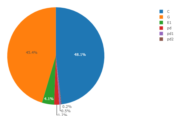
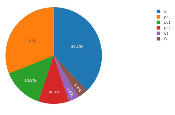
For further exploration, the data can also be visualized. The following three plots will show: (i) a boxplot of frequencies for each waveform type, (ii) a pie chart of time spent in each waveform type (iii) a pie chart showing the number of each waveform type.
epgminer::plot_fbox(example_epg_labeled)
epgminer::plot_pie(example_epg_labeled, pietype = "time")
epgminer::(example_epg_labeled, pietype = "number")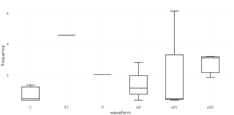
Expected Output and Run time
Expected output for each step is as follows:
Frequency and Relative Amplitude are calculated for each waveform instance and returned in a table. The frequency object is a table with columns for waveform and frequency, while the RA object is a table with columns for waveform, mean volts, SD of volts and Relative Amplitude.
Expected output is two summary tables for frequency and Relative Amplitude grouped by waveform respectively. There should be one (mean) frequency and (mean) Relative Amplitude for each waveform type.
Three plots where the first is a boxplot of frequencies and the last two are pie charts by time and number respectively.
Overall expected run time for this demo, not including package installation, is less than 1 minute.